Never Have I Ever ... Won M6 competition?
My naïve year-long journey to the M6 competition

Introduction
M-series competition
M-series competition
M6 Competition
The M6 competition is a live financial forecasting competition that started in February 2022, and ended a year later in 2023. The competition followed duathlon approach consisting of forecasting and investment tracks. For each track, the participants needed to submit (i) forecasts and (ii) investment decisions at each successive monthly submission point. The submission included forecasts and your investment strategy over the next four week period (normally 20 trading days). The competition data consisted from a universe of 50 S&P500 stocks and 50 ETFs, covering a variety of asset categories.
The forecasting performance for a particular submission point was measured by the Ranked Probability Score (RPS). The score evaluated the skills of the forecasting models to predict the ranking, from 1 (worst performing) to 5 (best performing), of realised percentage total returns of all assets (stocks and ETFs) over the forecasting period. The performance of the investment decisions was measured by means of a variant of the Information Ratio (IR), defined as the ratio of the portfolio return, ret, to the standard deviation of the portfolio return, sdp. Namely, risk adjusted returns are defined as \(IR = {ret}/{sdp}\). More details on the rules of the competition are available in guidlines.
My journey in the M6 competition started in January 2022, when I first heard about the competition. I considered the competition as a good sandbox to test my forecasting and optimization skills and hopefully build on it further learning from the best in the field. The beginning of the competition coincided with my moving process from a PhD life to an industry job in Belgium. Thanks to Belgian bureaucracy, I had some time in the beginning of the competition to experiment but later in time I felt into more straightforward let-see-what-I-can-do-the-day-before-the-submission approach. Nevertheless, It was fun and I learned a lot. I hope that this post will be compelling for other participants of the competition and for the readers in general.
Disclaimer: I had close-to-zero knowledge of financial markets at the start, so please take my comments with a grain of salt. Actually, the team names says it all: AM naïve.
Forecasting
I had big hopes for the forecasting track but the first results were not promising. At first, I was experimenting with statistical models using Darts python library. The method was to find a local (one model - one target time series) or global (one model - multiple target time series) model that would provide the asset return forecast over 20 days horizon. Normally, the base mode was Lasso or Ridge model. Then I used the quantiles of the forecasting residuals to define the rank of the time series. This approach was very naive and way far from the top. Actually, one of the reasons was the wrong interpretation of the rules how ranking is done. For some reason, I thought that the ranking among the ETF and stock classes should be different.
The first failures motivated me to go to the extreme. It was a time of Deep Learning and Transformer models. I modified the Temporal Fusion Transformer from pytorch-forecasting library to predict the quantiles the assets for the next 20 days. Although the results improved, the benchmark was not overcomed. Somewhere at this stage I switched to the investment part of the competition because I got some chances to win the quarterly prize. So, for some months I used the benchmark submission before I came back to the forecasting track with an idea of Multivariate Convolutional Neural Network, where instead of images at specific channels I used multivariate time series data of the assets. In contrast to the case with the transformer, the model would directly predict the quantiles of the assets in 20 days from now and possible reduce error accumulation. However, no luck with this model as well.
In the end, it was a question of honor to beat the benchmark (the score of the benchmark is 0.16) before the end of the competition. To do so, I decided to use the superpower of all Kagglers – LightGBM model. The idea was to use the LightGBM model as a multi-class classification model to predict the asset ranking in 20 days. Interestingly, the #2 place of the competition also used the decision tree but with multi-label classification. Read why it was preferred over multi-class classification in Miguel Perez Michaus post. To calibrate the probabilities of a given model, I’ve applied an isotonic recalibration combined with time series cross validation.
Did it work? This solution actually made my dream come true and I was able to beat the benchmark. I finished 16th out of 223 in the forecasting track in Quarter 4 of the competition. However, I was curious if this model could actually let me win the whole competition conditioned that I was using it from the beginning. So I decided to backtest the model and see how it would perform.
Backtesting LightGBM
The benchmarking was done with LightGBM without calibration as using the latter gave slightly worse performance results. The backtesting suggests that LightGBN would achieve 0.157623 in RPS. This score would allow me to finish in top 10 of the forecasting track. Below, you can see that the backtesting results per month and quarter. The divergence between the train and test results suggest that the model has overfitting issues that could have been dealt with. However, the model was not tuned and the main goal was to see if the model could be competitive.
Feature importance
Another interesting thing for me was to look at the features that the model found useful. Overall, I used the following features:
- Custom trading strategy with several indexes (SMA, EMA, RSI, MACD, etc.)
- Features based on the transformation of stock prices, volumes
- Categorical features based on the ticker properties (sector, industry, etc.)
- One hot encodings of holidays
- Spline of day of the week
- Kernels for holidays
Below, you can see the feature importance by split and gain. In both cases, the most important time series features were Simple Moving Average of trading Volume over 20 days, Cumulative Percentage Returns over 20 days, and Logarithmic Return over 20 days. The most important categorical features were asset class and asset type.
Investment
In the first quarter, simple method was used of minimizing risk with a given minimal level of returns. This method showed good results during the pilot submission but later providing mostly negative IR. At this stage, I have used the residuals of the forecasting model for the covariance matrix and mean values. Disappointed by the results, I came across Riskfolio-Lib. The library is amazing but without a good understanding of the theory behind the methods, it is hard to use it. So, my solution to this dilemma was to use the library as a black box and try to find the optimization method that provides the best investment returns. The summary of the approach you can see below.
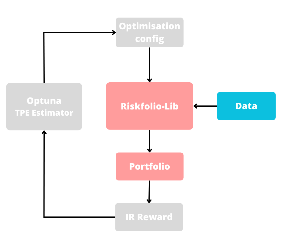
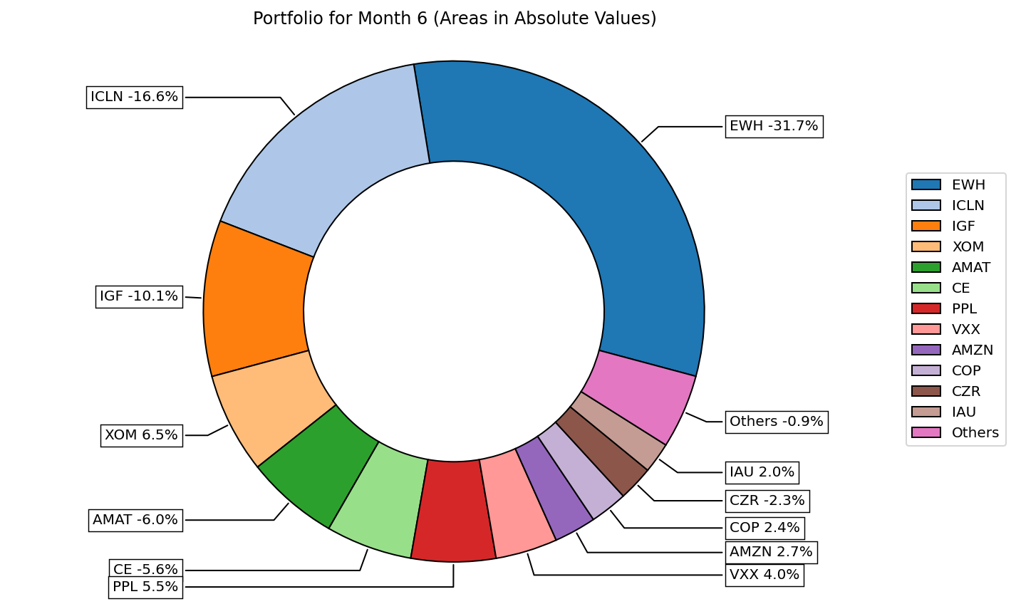
The first attempt was a failure, strictly speaking. I finished second … from the bottom. On the day of the submission for the next month #4 I was doing some adjustments and missed the deadline by several minutes. That was an unpleasant experience. However, as they say everything is all for the best. Luckily, the rules of the competition are such that if you miss the submission, the results from the previous month are forwarded to the next. To my surprise, the solution that was the second from the bottom in month #3 became the first in month #4. At this moment, I felt that there is some chance to win something so I decided to push more effort into the investment part of the competition. I kept 11th in the month #5 but fell to #162 in the month #6 going below zero IR. In the next quarter, I started promising by finishing #17 in month #7 and #7 in month #8. However, month #9 was unlucky for me as I finished #162. Unfortunately, two good months and one extremely bad month dropped me at #24 place in Q3 quarter.
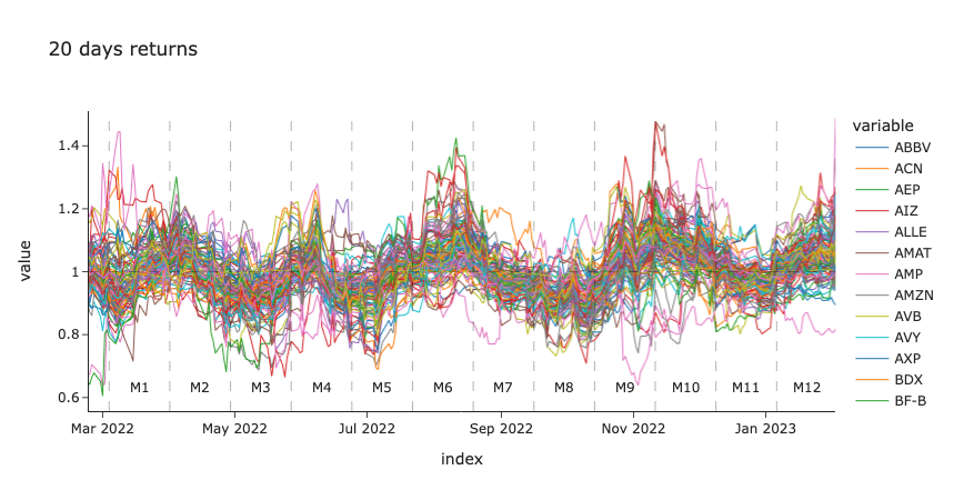
For the last quarter, I have noticed that there is a seasonality in the 20 days returns as shown in the figure below. So, I have tried to use the estimated trend in the portfolio optimization by training the portfolio on the months with same dynamics as the current month. However, this approach did not work well for me as I finished #152 in Q4 with negative IR.
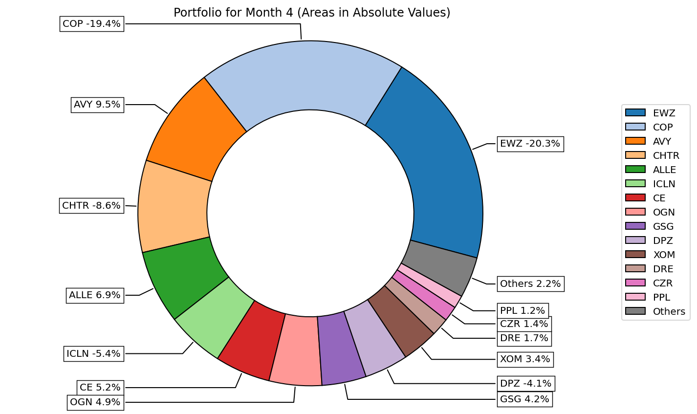
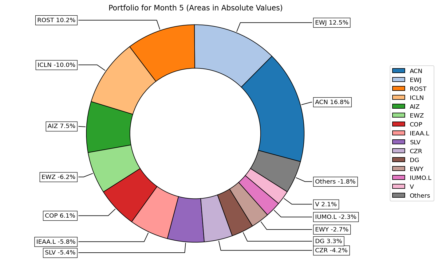
Looking back at the relative success (luck?) of the investment part for me, I think one of the reasons for good IR in Q2 and Q3 was the fact the ratio of short positions over long was prevailing in my portfolio. So these summer months were aligned with my strategy. The portfolios for the second quarter are shown below.
Conclusion
The competition was an amazing experience that kept me excited during the whole year. I thank the organizers for a wonderful competition and their efforts. One drawback for me is that despite more than 200 teams participated in the competition, the community was less active than I had expected or you could see on Kaggle. However, the good thing is that you can read the stories of the other participants here:
- The Options Market Beat 97.6% of Participants in the M6 Financial Forecasting Contest
- FinQBoost: Machine Learning for Portfolio Forecasting
- How I won $6,000 in the M6 Forecasting Competition
The code for this post and my solution is available on github:

